Dijkstras++

08-19-2025·7 min read

Context

A few days ago a group of researchers released a paper detailing an algorithm that surpasses any single-source shortest path algorithm in terms of time complexity. Before we dive into the details, it's important that we develop a good understanding of the current landscape of these algorithms. Unless you cheated your way through data structures (or just are not a Computer Science student), then you have heard of Dijkstras algorithm. Hopefully, you have also heard of Bellman-Ford as well, although this one is marginally less popular. Both of these algorithms are, or were, considered to be the best options to find the shortest path from one vertexHence, single-source shortest-path, V, on a graph to another vertex on the graph.

At a high level, Dijkstras works like this: from a given starting point, traverse all edges and keep track of the weight of that edge. Then for every vertex you visit, check your accumulated distance travelled. If the vertex has a lower distance travelled, then you know that the path you took to get there is not the shortest. Conversely, if you reach a node and the distance the node has stored is greater than your accumulated distance, then you know that your current path is the shortest (so far). This is pretty intuitive, but heres a picture anyways: 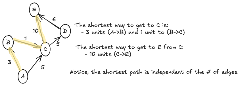Simple Dijkstras Flow

Bellman-Ford is a little bit less intuitive as it is meant to handle a corner case: negative edge weights. If we think back to how Dijkstras works, you'll notice that in the case where you have 3 vertices connected by negative weightsOr, at the very least the cycle between these 3 vertices have edge weights that sum to $< 0$ , there is nothing stopping the algorithm from continuously looping through this cycle until it has a weight of negative infinity, thus guaranteeing the shortest path. This case is solved in Bellman-Ford. Instead of just doing one pass through the graph, this algorithm iterates multiple times over each vertex. The key insight is that any true shortest path can use at most $V−1$ edgesWhere $V$ is the total number of vertices in the graph since any more edges would signify a repeating vertex and thus a cycle. So Bellman-Ford iterates over all vertices $V-1$ times and updates the shortest distance to every other vertex similar to how Dijkstras does. The kicker is that it runs one final iteration (the $Vth$ iteration) to see if any paths can still be improved. If a path can still be improved at this last iteration, there must be a negative weight cycle somewhere.

The last thing we need to understand before diving into the paper is the time complexity of these algorithms. Since Dijkstras goes through every vertex and edge in the graph while maintaining the "closest" vertices with a min-heap, it has a runtime of $O(V log V)$ At every vertex spend $log V$ time adding to the heap. On the other hand, Bellman-Ford iterates over all edges $V$ times, so the time complexity is $O(VE)$ .

Breaking the Barrier

Now that the context is (hopefully) clear, lets see how a team of researchers beat the status-quo. Since the implementation of Dijkstras uses a heap, which they refer to as the frontier $S$ , to track the minimum distance to given vertices, the team derived two key insights:

A vertex is "complete" if its true minimum distance has been found
If a vertex is "incomplete" then its shortest path is dependent on a complete vertex in the heap (or a vertex in the heap that will be complete before the current one). It follows that the best way to optimize Dijkstras is by minimizing the frontier, which is where Bellman-Ford comes in.

Given an arbitrary upper bound $B$ , we can define $U$ as the set of all vertices that have a minimum length $< B$ and the shortest path between the source and that vertex go through some vertex in $S$ . Then, select a parameter $k$ such that $k = log^{\Omega{(1)}} n$ to be a threshold between choosing to run Bellman-Ford or Dijkstras on the set of vertices in $S$ . Formally, there are two cases:

$|U|/k > |S|$ -> $S$ , the frontier, is already small enough.
$|U|/k \leq |S|$ -> $S$ is too large.

When $S$ is too large, it can be decreased by $k$ iterations of Bellman-Ford from vertices in $S$ . By doing so, all vertices with a shortest path from a vertex in $S$ that has $< k$ edges will be "complete". This will leave $|U|/k$ vertices, or pivotsThe vertices leftover are referred to as pivots since the shortest path to other vertices depends on them, putting us at the same size frontier as the first condition.

Bounded Multi-Source Shortest Path

Now that the frontier is reasonably small ( $< |U|/k$ ), the algorithm employs a recursive divide-and-conquer approach to handle the frontier. But what is it dividing and conquering? Suppose the set of vertices, $U$ , is partitioned into $2^t$ pieces where the partitioned sets contain vertices of similar size. By recursively dividing these sets, the algorithm will reach the base case where each partition is a singletonA set with size equal to 1 after $\frac{\log{n}}{t}$ levels. Every level is $\frac{n}{2^{kt}}$ sizeThis is obvious if you calculate the size of each partition for levels 1, 2, 3, etc., where $k$ is the number of levels. Setting this relation equal to one and solving for $k$ gets the above result of $\frac{\log{n}}{t}$

Each of these partitions, or subproblems that the algorithm divides up, are solved via BMSSP, or Bounded Multi-Source Shortest Path. It sounds like a mouthful, but really all it is is a reiteration of the logic already discussed. To clear up any confusion, suppose you have a distance $b$ . The current stage you are on, you know that if a vertex with shortest path $< b$ is complete (as we have said). As a corollary, this means that every vertex with shortest path $\geq b$ is incomplete and relies on a complete vertex in the frontier. Hence, we arrive at a relationship: $b \leq d(v) < B$ which is the motivation behind BMSSP. Thus, all this subproblem comes out to is finding the shortest path from the complete vertices in the frontier to a given vertex.

We're still missing one very large aspect of the algorithm, what exactly is $B$ ? All the way back at the start of this section, $U$ was defined as "the set of all vertices that have a minimum length of $< B$ . By the nature of the fundamental edge of the algorithm, it should be clear that $B$ is not a constant value. Instead, it adjusts at each level. Well, its important to know that BMSSP takes in three parameters:

Frontier $S$ , with invariant: $|S| \leq 2^{lt}$
Bound $B$ , with invariant: $B > max(\hat{d}(x))$ for $x$ in $S$
Level $l$ , with invariant: $0 \leq l \leq \frac{\log{n}}{t}$

Given specific arguments, BMSSP will return $B`$ , (where $B` \leq B$ ) as well as set $U`$ with where all vertices in $U`$ have a true distance less than $B`$ . Furthermore, there are two cases here. First, $B` = B$ , in which case the subroutine is complete. Otherwise, $B` < B$ , in which case it will recurse further. Essentially, the algorithm is initialized with $B = \infty$ and $B`$ progressively narrows and the frontier is progressively reduced until a shortest path is found.

The beauty of divide-and-conquer approaches lies in the fact that you really only have to look at a couple of different cases. Recursion in general is very elegant because once you are able to get away from the overhead in thinking about it, it becomes a simple proof of induction, but I digress. A key function of this algorithm is that it has a FindPivots() function that analyzes the frontier elements to look for pivotsThe roots of the shortest-path trees currently being searched for vertices.

Conclusion

Combining all of these ideas together, along with some more complex mathematics and recurrence relationships out of the scope of this blog, we will get an algorithm that deterministically finds the single-source shortest path in $O(m \log^\frac{2}{3}n)$ time. While this complexity only amounts to a (relatively) slow speedup, the intricacy is hard to deny. All of these techniques are designed to reduce the time spent at each vertex from $\log{n}$ to a lower value, which is what we see here. As with many things in life, there is no substitute to interacting with the material yourself with the paper here.